Non-uniform signal axes

LumiSpy facilitates the use of non-uniform axes, where the points of the axis vector are not uniformly spaced. This situation occurs in particular when converting a wavelength scale to energy (eV) or wavenumbers (e.g. for Raman shifts).

The conversion of the signal axis can be performed using the functions to_eV(), to_invcm() and to_raman_shift() (alias for to_invcm_relative()). If the unit of the signal axis is set, the functions can handle wavelengths in either nm or µm.

Accepted parameters are inplace=True/False (default is True), which determines whether the current signal object is modified or a new one is created, and jacobian=True/False (default is True, see Jacobian transformation).

The energy axis

The transformation from wavelength \(\lambda\) to energy \(E\) is defined as \(E = h c/ \lambda\). Taking into account the refractive index of air and doing a conversion from nm to eV, we get:

\[E[eV] = \frac{10^9}{e}\frac{h c}{n_{air} \lambda[nm]},\]

where \(h\) is the Planck constant, \(c\) is the speed of light, \(e\) is the elementary charge and \(n_{air}\) is the refractive index of air, see also [Pfueller].

>>> s2 = s.to_eV(inplace=False)
>>> s.to_eV()

Note

The refractive index of air \(n_{air}\) is wavelength dependent. This dependence is taken into account by LumiSpy based on the analytical formula given by [Peck] valid from 185-1700 nm (outside of this range, the values of the refractive index at the edges of the range are used and a warning is raised).

The wavenumber axis/Raman shifts

The transformation from wavelength \(\lambda\) to wavenumber \(\tilde{\nu}\) (spatial frequency of the wave) is defined as \(\tilde{\nu} = 1/ \lambda\). The wavenumber is usually given in units of \(\mathrm{cm}^{-1}\).

When converting a signal to Raman shift, i.e. the shift in wavenumbers from the exciting laser wavelength, the laser wavelength has to be passed to the function using the parameter laser using the same units as for the original axis (e.g. 325 for nm or 0.325 for µm) unless it is contained in the LumiSpy metadata structure under Acquisition_instrument.Laser.wavelength.

TODO: Automatically read laser wavelength from metadata if given there.

>>> s2 = s.to_invcm(inplace=False)
>>> s.to_invcm()
>>> s2 = s.to_raman_shift(inplace=False, laser=325)
>>> s.to_raman_shift(laser=325)

Jacobian transformation

When transforming the signal axis, the signal intensity is automatically rescaled (Jacobian transformation), unless the jacobian=False option is given. Only converting the signal axis, and leaving the signal intensity unchanged, implies that the integral of the signal over the same interval would lead to different results depending on the quantity on the axis (see e.g. [Mooney] and [Wang]).

For the energy axis as example, if we require \(I(E)dE = I(\lambda)d\lambda\), then \(E=hc/\lambda\) implies

\[I(E) = I(\lambda)\frac{d\lambda}{dE} = I(\lambda)\frac{d}{dE} \frac{h c}{E} = - I(\lambda) \frac{h c}{E^2}\]

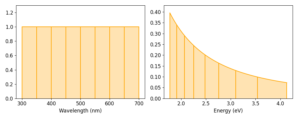
The minus sign just reflects the different directions of integration in the wavelength and energy domains. The same argument holds for the conversion from wavelength to wavenumber (just without the additional prefactors in the equation). The renormalization in LumiSpy is defined such that the intensity is converted from counts/nm (or counts/µm) to counts/meV. The following figure illustrates the effect of the Jacobian transformation:

Transformation of the variance

Scaling the signal intensities implies that also the stored variance of the signal needs to be scaled accordingly. According to \(Var(aX) = a^2Var(X)\), the variance has to be multiplied with the square of the Jacobian. This squared renormalization is automatically performed by LumiSpy if jacobian=True. In particular, homoscedastic (constant) noise will consequently become heteroscedastic (changing as a function of the signal axis vector). Therefore, if the metadata.Signal.Noise_properties.variance attribute is a constant, it is converted into a hyperspy.signal.BaseSignal object before the transformation.

See Signal variance (noise) for more general information on data variance in the context of model fitting and the HyperSpy documentation on setting the noise properties.

Note

If the Jacobian transformation is performed, the values of metadata.Signal.Noise_properties.Variance_linear_model are reset to their default values (gain_factor=1, gain_offset=0 and correlation_factor=1). Should these values deviate from the defaults, make sure to run hyperspy.signal.BaseSignal.estimate_poissonian_noise_variance() prior to the transformation.